library('here')library('dplyr')source(here("R/getAllData.R"))# read from all source files# full_df <- getAllData() %>%# mutate(# source = program,# site = Monitoring.Location.ID,# datetime = Activity.Start.Date.Time,# analyte = DEP.Analyte.Name,# value = DEP.Result.Value.Number,# units = DEP.Result.Unit,# latitude = Org.Decimal.Latitude,# longitude = Org.Decimal.Longitude,# sample_depth = Activity.Depth,# .keep = "none"# )# read from cached file produced by index.qmdfull_df <-read.csv(here("data", "exports", "dashboardData.csv"))df <-filter(full_df, analyte == params$analyte)
create .csv of analyte data
# save df to csv# reduce to only cols we need & save to csvdf %>%write.csv(here("data", "exports", "unified-wq-db-samples", paste0(params$analyte, ".csv")))
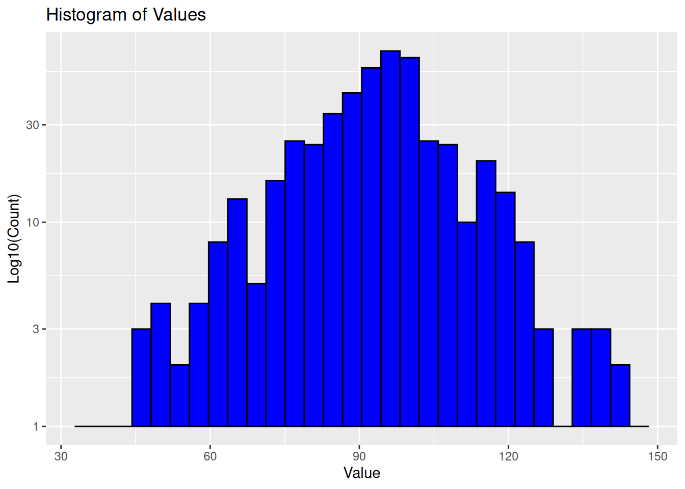
value Distribution Across All Datasets
display histogram of values
library(ggplot2)ggplot(df, aes(x = value)) +geom_histogram(bins =30, fill ="blue", color ="black") +scale_y_log10() +labs(title ="Histogram of Values", x ="Value", y ="Log10(Count)")
Note that values are often not directly comparable due to the use of different units.
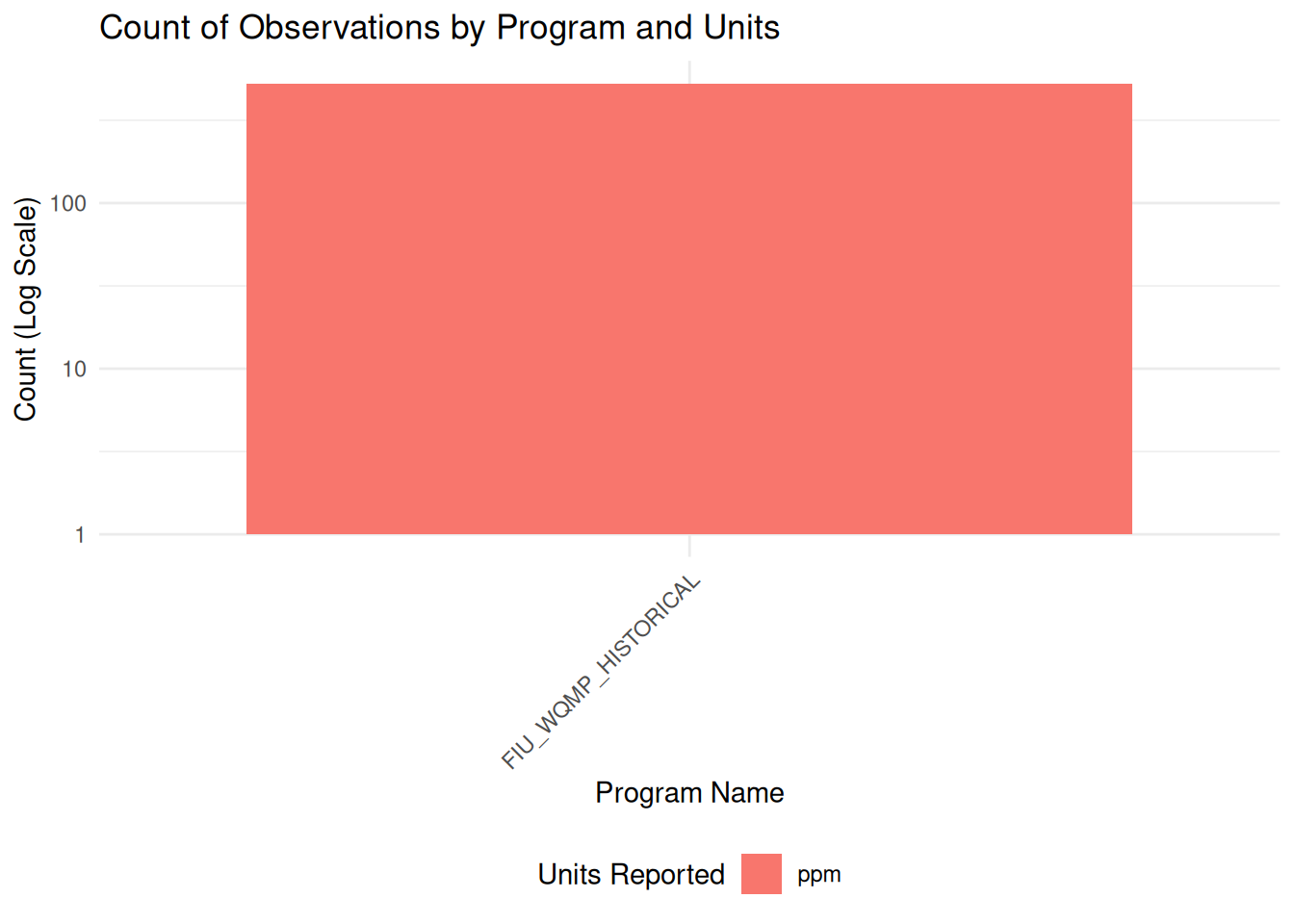
Show units used by each program
library(ggplot2)ggplot(df, aes(x = source, fill = units)) +geom_bar() +scale_y_log10() +labs(title ="Count of Observations by Program and Units",x ="Program Name",y ="Count (Log Scale)",fill ="Units Reported" ) +theme_minimal() +theme(legend.position ="bottom",axis.text.x =element_text(angle =45, hjust =1) )
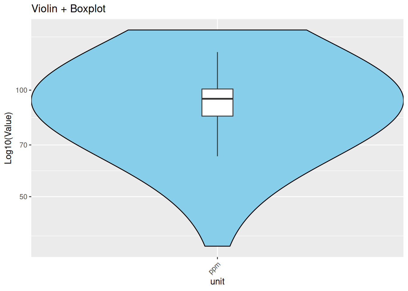
Show values grouped by units
library(ggplot2)ggplot(df, aes(x = units, y = value)) +geom_violin(width =1.2, adjust =10, fill ="skyblue", color ="black") +geom_boxplot(width =0.1, outlier.shape =NA) +scale_y_log10() +theme(axis.text.x =element_text(angle =45, hjust =1)) +labs(x ="unit", y ="Log10(Value)", title ="Violin + Boxplot")
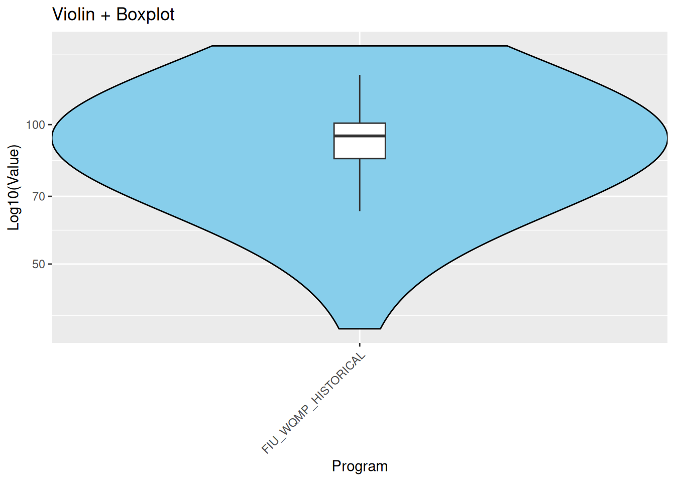
Values Reported By Program:
Show value distributions for each program
library(ggplot2)ggplot(df, aes(x = source, y = value)) +geom_violin(width =1.2, adjust =10, fill ="skyblue", color ="black") +geom_boxplot(width =0.1, outlier.shape =NA) +scale_y_log10() +theme(axis.text.x =element_text(angle =45, hjust =1)) +labs(x ="Program", y ="Log10(Value)", title ="Violin + Boxplot")
Station Statistics:
create station statistics dataframe
source(here("R/seasonalMannKendall.R"))library(lubridate) # for mdy_hms()library(pander) # for display# create table of samples for each stationsamples_df <- df %>%# drop any with empty Monitoring.Location.IDfilter(!is.na(site)) %>%# drop any with empty Activity.Start.Date.Timefilter(!is.na(datetime)) %>%# parse the "YYYY-MM-DD" strings into POSIXctmutate(datetime =ymd( datetime,tz ="UTC")) %>%distinct()# add statistics for each stationsample_stats_df <- samples_df %>%group_by(source, site) %>%reframe( { tmp <-seasonalMannKendallVectorized( datetime, value ) },n_values =n(),mean =mean(value),min =min(value),max =max(value),coefficient.of.variation =sd(value) /mean(value) ) %>%mutate(# create column significant_slopesignificant_slope =ifelse(z <=0.05, slope, NA_real_),pvalue = z ) %>%# drop unwanted columns added by seasonalMannKendallselect(-z,-tau,-chi_square )# print(head(sample_stats_df))# # display sample_stats_df with pander# pander(sample_stats_df)
library(gt)library(scales)library(tidyselect) # for all_of()library(RColorBrewer) # for brewer.pal()# ── color_column() ─────────────────────────────────────────────────────────────# gt_tbl : a gt object that you’ve already created (e.g. `sample_stats_df %>% gt()`)# df : the original data.frame (must contain the column you want to color)# column : a string, e.g. "slope" or "n_values"# palette : a character vector of colours to feed to col_numeric()#color_column <-function(gt_tbl, df, column, palette =c("red", "orange", "yellow", "green", "blue", "violet"),domain =NULL) {# 1) Pull out that column’s numeric values vals <- df[[column]]if (!is.numeric(vals)) {stop(sprintf("`%s` is not numeric; data_color() requires a numeric column.", column)) }# 2) Compute its min and max (ignoring NA) min_val <-min(vals, na.rm =TRUE) max_val <-max(vals, na.rm =TRUE)if (is.null(domain)) { domain <-c(min_val, max_val) }# 3) Call data_color() on the gt table for that single column gt_tbl %>%data_color(columns =all_of(column),colors =col_numeric(palette = palette,domain = domain ) )}library(dplyr)library(gt)# 1) First build your gt table as usual:gt_tbl <- sample_stats_df %>%gt()# slope blue (-) to red (+) (0 centered)tryCatch({ min_slope <-min(sample_stats_df$slope, na.rm =TRUE) max_slope <-max(sample_stats_df$slope, na.rm =TRUE) max_abs_slope <-max(abs(min_slope), abs(max_slope)) gt_tbl <-color_column( gt_tbl, df = sample_stats_df, column ="slope",palette =rev(brewer.pal(11, "RdBu")),domain =c(-max_abs_slope, max_abs_slope) )}, error =function(e) {print("Error in slope color column")print(e)})tryCatch({# pvalue Z gt_tbl <-color_column( gt_tbl, df = sample_stats_df, column ="z", palette = scales::brewer_pal(palette ="Blues")(9) )}, error =function(e) {print("Error in z color column")print(e)})
[1] "Error in z color column"
<simpleError in color_column(gt_tbl, df = sample_stats_df, column = "z", palette = (scales::brewer_pal(palette = "Blues"))(9)): `z` is not numeric; data_color() requires a numeric column.>
display with gt
# slope blue (-) to red (+) (0 centered)tryCatch({ min_slope <-min(sample_stats_df$significant_slope, na.rm =TRUE) max_slope <-max(sample_stats_df$significant_slope, na.rm =TRUE) max_abs_slope <-max(abs(min_slope), abs(max_slope)) gt_tbl <-color_column( gt_tbl, df = sample_stats_df, column ="significant_slope",palette =rev(brewer.pal(11, "RdBu")),domain =c(-max_abs_slope, max_abs_slope) )}, error =function(e) {print("Error in significant_slope color column")print(e)})
[1] "Error in significant_slope color column"
<rlang_error in col_numeric(palette = palette, domain = domain): Wasn't able to determine range of `domain`>
display with gt
tryCatch({# mean values blue to red (0 centered) min_mean <-min(sample_stats_df$mean, na.rm =TRUE) max_mean <-max(sample_stats_df$mean, na.rm =TRUE) max_abs_mean <-max(abs(min_mean), abs(max_mean)) gt_tbl <-color_column( gt_tbl, df = sample_stats_df, column ="mean",palette =rev(brewer.pal(11, "RdBu")),domain =c(-max_abs_mean, max_abs_mean) )}, error =function(e) {print("Error in mean color column")print(e)})tryCatch({# n values white to green gt_tbl <-color_column( gt_tbl, df = sample_stats_df, column ="n_values", palette = scales::brewer_pal(palette ="Greens")(9) )}, error =function(e) {print("Error in n_values color column")print(e)})tryCatch({# min gt_tbl <-color_column( gt_tbl, df = sample_stats_df, column ="min", palette = scales::brewer_pal(palette ="Blues")(9) )}, error =function(e) {print("Error in min color column")print(e)})tryCatch({# max gt_tbl <-color_column( gt_tbl, df = sample_stats_df, column ="max", palette = scales::brewer_pal(palette ="Blues")(9) )}, error =function(e) {print("Error in max color column")print(e)})tryCatch({# coefficient.of.variation gt_tbl <-color_column( gt_tbl, df = sample_stats_df, column ="coefficient.of.variation", palette = scales::brewer_pal(palette ="Blues")(9) )}, error =function(e) {print("Error in coefficient.of.variation color column")print(e)})# 4) Render/display:gt_tbl